For \(m,n\in \mathbb{N}\) let \(\beta_{m,n}\colon m+n\rightarrow n+m\) be the morphism in \(h_1 \mathrm{K}^b_{\mathrm{loc}}(\mathrm{Sbim})\) given by the chain homotopy class of the shifted Rouquier complex \((X_{m,n})\) defining the cabled crossing in Definition 2.2.7.
2.5 Prebraiding for Soergel bimodules[001V]
We are now prepared to construct a prebraiding on the functor \(h_1 K_{\mathrm{loc}}\colon h_1 \mathrm{BSbim}\rightarrow h_1 \mathrm{K}^b_{\mathrm{loc}}(\mathrm{Sbim})\) from ([001D]).
Theorem 2.5.2. (Prebraiding for Soergel bimodules).
The family of morphisms \(\beta_{m,n}\) from Definition 2.5.1 constitute a prebraiding on the functor \(h_1 K_{\mathrm{loc}}\colon h_1 \mathrm{BSbim}\rightarrow h_1 \mathrm{K}^b_{\mathrm{loc}}(\mathrm{Sbim})\).
Considering \(h_1 K_{\mathrm{loc}}\colon h_1 \mathrm{BSbim}\rightarrow h_1 \mathrm{K}^b_{\mathrm{loc}}(\mathrm{Sbim})\) as a functor over \(h_1\mathrm{DMor}^{\mathrm{poly}, \mathrm{gr-perf}}(\mathrm{mod}_k^{\mathbb{Z}})\) via the functor \(h_1H_{\mathrm{loc}}\colon h_1 \mathrm{K}^b_{\mathrm{loc}}(\mathrm{Sbim}) \rightarrow h_1\mathrm{DMor}^{\mathrm{poly}, \mathrm{gr-perf}}(\mathrm{mod}_k^{\mathbb{Z}})\), we obtain the following refined version:
Corollary 2.5.3. (Relative prebraiding on \(h_1 K_{\mathrm{loc}}\)).
The Rouquier complexes of cabled crossings define a prebraiding on \(h_1 K_{\mathrm{loc}}\colon h_1 \mathrm{BSbim}\rightarrow h_1 \mathrm{K}^b_{\mathrm{loc}}(\mathrm{Sbim})\) over \(h_1\mathrm{DMor}^{\mathrm{poly}, \mathrm{gr-perf}}(\mathrm{mod}_k^{\mathbb{Z}})\).
Proof.
By Remark 2.2.6, the braiding complexes are quasi-isomorphic to the associated permutation bimodules, concentrated in homological degree \(0\). As the permutation bimodules implement the symmetric braiding, this means that the braiding complexes constructed as (shifted) Rouquier complexes of the cabled crossings become the canonical symmetric braiding in \(h_1\mathrm{DMor}^{\mathrm{poly}, \mathrm{gr-perf}}(\mathrm{mod}_k^{\mathbb{Z}})\). ◻
The following result is the crucial naturality part for the proof of Theorem 2.5.2. The result is in fact stronger than needed, since it is a statement on the chain level.
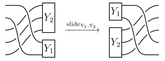
For any Bott–Samelson bimodule of the form \(Y=Y_1\boxtimes Y_2\) in \(\mathrm{BSbim}_m\boxtimes \mathrm{BSbim}_n\subset \mathrm{Sbim}_{m+n}\), there are homotopy equivalences of chain complexes in \(\mathrm{Ch}^b(\mathrm{Sbim}_{m+n})\): \[\begin{aligned} \mathrm{slide}_{Y_1,Y_2}\colon & X_{m,n} \circ_1Y \longrightarrow \mathrm{swap}_{m,n}(Y)\circ_1X_{m,n} \end{aligned}\]
We also use the notation \(\mathrm{slide}_{Y}\coloneqq\mathrm{slide}_{Y_1,Y_2}\), when \(m\) and \(n\) are clear from the context.
Proof of theorem 2.5.2.
theorem 2.5.4 indeed implies theorem 2.5.2. Namely it follows from Theorem 2.2.4 that the \(\beta_{m,n}\) are invertible and satisfy the hexagon axioms ([001L]) and thus form the components of a natural transformation \(\boxtimes\circ (h_1 K_{\mathrm{loc}}\times h_1 K_{\mathrm{loc}}) \Rightarrow \boxtimes^{\mathrm{op}}\circ (h_1 K_{\mathrm{loc}}\times h_1 K_{\mathrm{loc}})\) by Theorem 2.5.4. ◻
To establish theorem 2.5.4 we construct, after some preparation, the chain maps, which we then call slide maps, explicitly. For this we work with the Hecke category \(\mathcal{DS}_n\), i.e. the diagrammatical presentation of the monoidal \(1\)-category \(\mathrm{BSbim}_n\) from [EW16], [EK10]. The construction of the chain maps \(\mathrm{slide}_{Y_1,Y_2}\) proceeds in two steps. The first step is specific to the setting of Bott–Samelson and Soergel bimodules and uses \(\mathcal{DS}\). It establishes the existence of atomic slide chain maps, namely \(\mathrm{slide}_{\mathbf{1}_1,B_1}\) for \((m,n)=(1,2)\) and \(\mathrm{slide}_{B_1,\mathbf{1}_1}\) for \((m,n)=(2,1)\); see Lemma 2.5.5. The second step uses that every Bott–Samelson bimodule is a composition (monoidal and horizontal) of Bott–Samelson bimodules on two strands, and so knowing the atomic slide chain maps is sufficient to construct general slide maps along the following scheme: 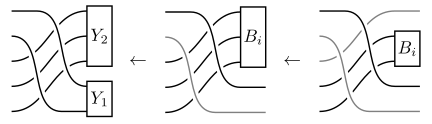 Essentially the same argument would work for any monoidal bicategory generated by a single object and one endomorphism of its tensor square.
To formulate the statements, we need at least a rough description of the Hecke category \(\mathcal{DS}_n\) and the fact that it is equivalent to \(\overline{\mathrm{BSbim}}^{\mathrm{gr}}_n\) as graded monoidal \(k\)-linear category. For details we refer to [EW16], [EK10]. Each simple reflection \(s_i\in S_n\) is encoded by a colour. Objects in \(\mathcal{DS}_n\) are finite ordered sequences of such colours and they encode the Bott–Samelson bimodules in the form ([000N]) (with \(j=0\) since we consider \(\overline{\mathrm{BSbim}}^{\mathrm{gr}}_n\)). For instance if \(n=2\) and we encode \(s_1\) as red and \(s_2\) as blue, then the Bott–Samelson bimodule \(B_{\mathbf{i}}\) from ([000N]) is encoded as a sequence of colors red and blue according to \({\mathbf{i}}\), for instance \({\mathbf{i}}=(1,1,2,1,1)\) corresponds to the object given by the color sequence \((red, red, blue, red, red)\). Morphisms in \(\mathcal{DS}_n\) are \(k\)-linear combinations of isotopy classes of certain decorated graphs embedded in the plane. A morphism from \(B_{\mathbf{i}}\) to \(B_{\mathbf{i}'}\) will have the colour sequence for \({\mathbf{i}}\) as bottom boundary and that for \({\mathbf{i}}'\) at the top boundary; for instance the first two diagrams in ([0023]) represent morphism from \((2,2)\) to \((2)\) and vice versa, the third goes from the unit to \((2)\), etc.
The monoidal structure is given on objects by concatenating sequences and, on morphisms, by (the bilinear extension of) placing diagrams horizontally next to each other. The composition of morphisms is, likewise, given by (the bilinear extension of) stacking diagrams on top of each other. The empty sequence is the unit object.
Apart from multiplication with polynomials, the generating morphisms (in the monoidal sense) are exactly the following, where blue represents any color/number which is neighbored to red and not neighbored to orange. 
For the rest of this section we identify \(\mathrm{BSbim}_n\) with \(\mathcal{DS}_n\) as monoidal \(1\)-categories (via \(\overline{\mathrm{BSbim}}^{\mathrm{gr}}_n\)) and perform computations using the diagrammatic calculus.
The Rouquier complexes ([000Z]) are translated into the diagrammatics as  where we encode \(s_i\) by blue. (Instead of remembering the grading shifts from ([000Z]), it is more convenient in the diagrammatic setting to consider the maps as homogeneous of degree one). To keep track of the monoidal unit (corresponding to \(R\)) appearing in the complexes, we mostly indicate them by a colored dot as shown in ([0024]).
There are slide chain maps 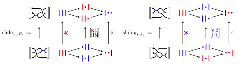 which are invertible up to homotopy. The inverses are given by the chain maps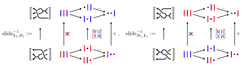
Proof.
The proof is given by an explicit calculation. As an example (the remaining cases are checked analogously) we show that \(\mathrm{slide}^{-1}_{\mathbf{1}_1,B_1}\circ\; \mathrm{slide}_{\mathbf{1}_1,B_1}\) is homotopic to the identity by computing their difference and exhibiting an explicit null-homotopy: 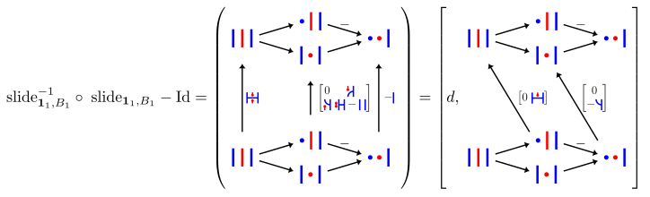 ◻
◻
Observe that the relevant chain complexes and chain maps are for the two cases are related by swapping the colours red and blue.
Readers familiar with the chain maps between Rouquier complexes associated to a Reidemeister III move will recognize the atomic slide chain maps as filtrations-preserving pieces of the former, see e.g. [MWW22, (3.3) and (3.4)].
Now that we have obtained the atomic slide chain maps in lemma 2.5.5, we can construct all remaining slide chain maps in an essentially formal way.
Proof of Theorem 2.5.4.
We will focus on the version for the positive cabled crossing, since the other one is analogous. First, we reduce to the case when the object \(Y=Y_1\boxtimes Y_2\) is a generating object of \(\mathrm{BSbim}_m\boxtimes \mathrm{BSbim}_n\). Otherwise, we can decompose into generators: \[Y_1\boxtimes Y_2= (Y_1\boxtimes \mathbf{1}) \circ_1(\mathbf{1}\boxtimes Y_2) = (B_{i_1}\boxtimes \mathbf{1}) \circ_1\cdots \circ_1(B_{i_a}\boxtimes \mathbf{1}) \circ_1(\mathbf{1} \boxtimes B_{j_1})\circ_1\cdots \circ_1(\mathbf{1} \boxtimes B_{j_b})\] and define \[\begin{aligned} \mathrm{slide}_{Y_1,\mathbf{1}}&:= (\mathrm{id}_{\mathrm{swap}_{m,n}(B_{i_1}\circ_1\cdots \circ_1B_{i_{a-1}} \boxtimes \mathbf{1})}\circ_1\mathrm{slide}_{B_{i_{a}},\mathbf{1}}) \circ_2\cdots \circ_2 (\mathrm{slide}_{B_{i_{1}},\mathbf{1}} \circ_1\mathrm{id}_{B_{i_1}\circ_1\cdots \circ_1B_{i_{a-1}} \boxtimes \mathbf{1}}) \\ \mathrm{slide}_{\mathbf{1},Y_2}&:= (\mathrm{id}_{\mathrm{swap}_{m,n}(\mathbf{1}\boxtimes B_{j_1}\circ_1\cdots \circ_1B_{j_{b-1}})}\circ_1\mathrm{slide}_{\mathbf{1}, B_{j_{b}}}) \circ_2\cdots \circ_2 (\mathrm{slide}_{\mathbf{1}, B_{j_{1}}} \circ_1\mathrm{id}_{\mathbf{1}\boxtimes B_{j_1}\circ_1\cdots \circ_1B_{j_{b-1}}}) \\ \mathrm{slide}_{Y_1,Y_2} &:= (\mathrm{id}_{\mathrm{swap}_{m,n}(Y_1\boxtimes \mathbf{1})} \circ_1\mathrm{slide}_{\mathbf{1},Y_2}) \circ_2(\mathrm{slide}_{Y_1,\mathbf{1}} \circ_1\mathrm{id}_{Y_2}) \end{aligned}\]
Now we turn to defining \(\mathrm{slide}_{B,\mathbf{1}_n}\) and \(\mathrm{slide}_{\mathbf{1}_m,B}\), where \(B\) is one of the generating Bott–Samelson bimodules. Here we place subscripts to distinguish the identity bimodules. We first consider the latter situation and reduce it to the case \(m=1\), where the cabled crossing is a Coxeter braid. Indeed, suppose that \(m>1\), then we use the first equality from Lemma 2.2.8 to define \(\mathrm{slide}_{\mathbf{1}_m,B}\) to be the composite: \[\begin{gathered} \nonumber \big((\mathrm{slide}_{\mathbf{1}_1,B}\boxtimes \mathrm{id}_{\mathbf{1}_{m-1}}) \circ_1\cdots \circ_1 \mathrm{id}_{\mathbf{1}_{m-1-i} \boxtimes X_{1,n}\boxtimes\mathbf{1}_{i}} \circ_1\cdots \circ_1 \mathrm{id}_{\mathbf{1}_{m-1}\boxtimes X_{1,n}}\big) \circ_2\cdots \\ \circ_2\big(\mathrm{id}_{X_{1,n}\boxtimes \mathbf{1}_{m-1}} \circ_1\cdots \circ_1 (\mathrm{id}_{\mathbf{1}_{m-1-i}} \boxtimes \mathrm{slide}_{\mathbf{1}_1,B}\boxtimes\mathrm{id}_{\mathbf{1}_{i}}) \circ_1\cdots \circ_1 \mathrm{id}_{\mathbf{1}_{m-1}\boxtimes X_{1,n}}\big) \circ_2\cdots\\ \nonumber \circ_2\big(\mathrm{id}_{X_{1,n}\boxtimes \mathbf{1}_{m-1}} \circ_1\cdots \circ_1 \mathrm{id}_{\mathbf{1}_{m-1-i} \boxtimes X_{1,n}\boxtimes\mathbf{1}_{i}} \circ_1\cdots \circ_1 (\mathrm{id}_{\mathbf{1}_{m-1}}\boxtimes \mathrm{slide}_{\mathbf{1}_1,B}) \big) \end{gathered}\] For the other case, we first choose chain maps \(\varphi\) and \(\varphi^{-1}\) realising the first homotopy equivalence in Lemma 2.2.8. Then we define \(\mathrm{slide}_{B,\mathbf{1}_n}\) as the composition: \[\begin{gathered} \nonumber \varphi^{-1} \circ_2\big((\mathbf{1}_{n-1}\boxtimes \mathrm{slide}_{B,\mathbf{1}_1}) \circ_1\cdots \circ_1 \mathrm{id}_{\mathbf{1}_{i} \boxtimes X_{m,1}\boxtimes\mathbf{1}_{n-1-i}} \circ_1\cdots \circ_1 \mathrm{id}_{X_{m,1}\boxtimes \mathbf{1}_{n-1}}\big) \circ_2\cdots \\ \circ_2\big(\mathrm{id}_{\mathbf{1}_{n-1}\boxtimes X_{m,1}} \circ_1\cdots \circ_1 (\mathrm{id}_{\mathbf{1}_{i}} \boxtimes \mathrm{slide}_{B,\mathbf{1}_1}\boxtimes\mathrm{id}_{\mathbf{1}_{n-1-i}}) \circ_1\cdots \circ_1 \mathrm{id}_{X_{m,1}\boxtimes \mathbf{1}_{n-1}}\big) \circ_2\cdots \\ \nonumber \circ_2\big(\mathrm{id}_{\mathbf{1}_{n-1}\boxtimes X_{m,1}} \circ_1\cdots \circ_1 \mathrm{id}_{\mathbf{1}_{i} \boxtimes X_{m,1}\boxtimes\mathbf{1}_{n-1-i}} \circ_1\cdots \circ_1 (\mathrm{slide}_{B,\mathbf{1}_1}\boxtimes \mathbf{1}_{n-1}) \big)\circ_2\varphi \end{gathered}\] It remains to construct \(\mathrm{slide}_{\mathbf{1}_1,B_i}\) and \(\mathrm{slide}_{B_j,\mathbf{1}_1}\) where \(B_i\) is a generating object of \(\mathrm{BSbim}_n\) and \(B_j\) is a generating object of \(\mathrm{BSbim}_m\). Now we reduce this problem to the cases when \(n=2\) and \(m=2\) respectively. We define \(\mathrm{slide}_{\mathbf{1}_1,B_i}\) as the composite: \[\begin{aligned} F(\sigma_{n}\cdots\sigma_{1}) \circ_1B_i =& F(\sigma_{n}\cdots\sigma_{i+1})\circ_1F(\sigma_{i}\sigma_{i-1})\circ_1F(\sigma_{i-2}\cdots\sigma_{1})\circ_1B_i \\ \rightarrow &F(\sigma_{n}\cdots\sigma_{i+1})\circ_1F(\sigma_{i}\sigma_{i-1}) \circ_1B_i \circ_1F(\sigma_{i-2}\cdots\sigma_{1}) \\ \xrightarrow{\mathrm{slide}} &F(\sigma_{n}\cdots\sigma_{i+1})\circ_1B_{i-1} \circ_1F(\sigma_{i}\sigma_{i-1}) \circ_1F(\sigma_{i-2}\cdots\sigma_{1}) \\ \rightarrow& B_{i-1} \circ_1F(\sigma_{n}\cdots\sigma_{i+1})\circ_1F(\sigma_{i}\sigma_{i-1}) \circ_1F(\sigma_{i-2}\cdots\sigma_{1})\\ =& B_{i-1} \circ_1F(\sigma_{n}\cdots\sigma_{1}) \end{aligned}\] where the unlabelled maps are far-commutativity isomorphisms and the labelled arrow is given by \(\mathrm{id}\circ_1\mathrm{slide}_{\mathbf{1}_1,B_1} \circ_1\mathrm{id}\), which is determined by the \(n=2\) case. The reduction of \(\mathrm{slide}_{B_j,\mathbf{1}_1}\) to the case \(m=2\) is completely analogous.
Thus we reduced the problem to the statement from Lemma 2.5.5. By construction, all slide maps constructed in this proof are homotopy equivalences. ◻
In Remarks 2.4.3 and 2.4.4 we have observed that a prebraiding need not satisfy the braid relation, and that the braid relation in prebraidings on identity functors can be verified in two ways using naturality. On the level of the homotopy category of Soergel bimodules, this is reflected in the fact, that the chain maps implementing the homotopy equivalence corresponding to a braid relation live in a 2-dimensional space [EK10, Section 3, Reidemeister 3 generators]. One dimension is encoding an overall non-zero scaling. Even after fixing this, there exists however a 1-dimensional affine subspace of representatives of the same homotopy class of chain maps. Two distinct (and thus spanning) points in this subspace can be built from slide chain maps, analogously to the two ways of establishing the braid relation in Remark 2.4.4.
We used Rouquier canonicity to ensure here the independence (up to canonical isomorphism) of our choices in the construction of the prebraiding on \(h_1 K_{\mathrm{loc}}\) in Theorem 2.5.2. For the rest of the paper it would be enough to make one of the choices and establish the prepraiding using only the monoidality of \(h_1 K_{\mathrm{loc}}\). The desired independence of choices (and in fact also Rouqiuer canonicity itself) could then be deduced from the existence statement in corollary 8.2.2.
Original source: arXiv:2401.02956v2
Original source · 2401.02956v2