The graded \(k\)-linear category of Bott–Samelson bimodules for \(R_n\) is the graded \(k\)-linear full subcategory \(\mathrm{BSbim}^{\mathrm{gr}}_n\) of \(R_n\)-bimodules given by all graded \(R_n\)-bimodules of the form: \[ B_{\mathbf{i}}\langle j\rangle:=R\otimes_{R^{s_{i_k}}}R\otimes_{R^{s_{i_{k-1}}}}\cdots\otimes_{R^{s_{i_1}}}R\langle j-k\rangle\] for \(R=R_n\), \(j\in\mathbb{Z}\) and some \(\mathbf{i}=(i_k,i_{k-1},\ldots, i_1)\in \{1,2,\ldots n-1\}^k\) with \(k \in \mathbb{N}_0\), including the bimodules \(R\langle j\rangle\) in case \(k=0\). In the case \(k=1\) we also abbreviate: \[B_i:= R\otimes_{R^{s_{i}}}R\langle-1\rangle\]
2 A prebraiding on the homotopy category of Soergel bimodules[000H]
2.1 Review of Soergel bimodules and diagrammatics[000I]
We let \(k\) denote the rationals \(\mathbb{Q}\) or, more generally, a commutative \(\mathbb{Q}\)-algebra. We consider the \(k\)-linear monoidal categories \(\mathrm{Sbim}_n\) of Soergel bimodules for the symmetric group \(S_n\) acting on its natural representation. In this section, if not specified otherwise, categories mean ordinary categories (in contrast to \(\infty\)-categories used later) and functors mean ordinary functors. For a fixed nonnegative integer \(n\), let \(R_n=k[x_1,x_2,\ldots, x_n]\) denote the polynomial ring over \(k\) in \(n\) variables viewed as polynomial functions on \(\mathfrak{h}^*=(k^n)^*\) in the standard way. Permuting the basis vectors of \(k^n\) induces a left action of the symmetric group \(W=S_n\) on \(R_n\) such that the simple transposition \(s_i=(i,i+1)\) acts by swapping the variables \(x_i\) and \(x_{i+1}\). Denote \(\check\alpha_i=x_{i}-x_{i+1}\) for \(1\leq i\leq n-1\). Then restriction to the span of the \(\check\alpha_i\)’s gives the usual geometric representation of \(W\) viewed as the Coxeter group generated by the simple transpositions. For any subgroup \(G\) of \(W\) let \(R_n^G\) be the subalgebra of \(G\)-invariants in \(R_n\). In case \(G=\langle s_i\rangle\) for some \(1\leq i\leq n-1\) we abbreviate \(R_n^G=R_n^i\). We will view \(R_n\) as a graded (by which we mean \(\mathbb{Z}\)-graded) algebra by putting the generators \(x_i\) in degree \(2\). Note that \(R_n^i\) is a graded subalgebra and we have a canonical, grading-preserving decomposition \[ R_n= R_n^i\oplus \check\alpha_iR_n^i\simeq R_n^i\oplus R_n^i\langle 2\rangle\] as graded \(R_n^i\)-bimodules. Here and in the following we denote for \(j\in \mathbb{Z}\) and a graded (bi)module \(M=\oplus_{i\in\mathbb{Z}} M_i\) by \(M\langle j\rangle\) the graded (bi)module which equals \(M\) as (bi)module but with the grading shifted up by \(j\), i.e. \(M\langle j\rangle_i=M_{i-j}\). The grading shifting functors \(\langle j\rangle\), \(j\in\mathbb{Z}\) equip the category of graded \((R_n,R_m)\)-bimodules for fixed \(n,m\) with an action of the group \(\mathbb{Z}\).
By a graded \(k\)-linear category11 we mean a category enriched in \(\mathbb{Z}\)-graded \(k\)-modules. As an example we can take as objects graded \(R_n\)-bimodules with all \(R_n\)-bimodule maps, denoted \(\mathrm{Hom}^{\mathrm{gr}}\). In this case, the grading shift functors are compatible with the grading on morphisms as follows: \[ \mathrm{Hom}^{\mathrm{gr}}(M\langle k\rangle,N\langle l\rangle) = \mathrm{Hom}^{\mathrm{gr}}(M,N)\langle l-k\rangle\]
Using this shorthand, ([000M]) may also be expressed as: \[ B_{\mathbf{i}}\langle j\rangle \simeq B_{i_k} \otimes_{R} B_{i_{k-1}}\otimes_R \cdots\otimes_R B_{i_1}\langle j\rangle\]
There are two common variations of definition 2.1.1: 
Namely, \(\mathrm{BSbim}_n\) is the \(k\)-linear (but no longer graded \(k\)-linear) category obtained by restricting to the degree zero part of the morphism spaces. We call this the degree zero subcategory. (In the language of enriched category theory, this is the underlying category of the category enriched in graded vector spaces; it inherits the linear structure.) By remembering the \(\mathbb{Z}\)-action by grading shift functors, all other homogeneous components of morphism spaces in \(\mathrm{BSbim}^{\mathrm{gr}}_n\) can be recovered from ([000K]).
Alternatively, one can consider the graded \(k\)-linear full subcategory \(\overline{\mathrm{BSbim}}^{\mathrm{gr}}_n\) on unshifted Bott–Samelson bimodules \(B_{\mathbf{i}}\), i.e. where \(j=0\) in ([000M]). From this category one can reconstruct the morphism spaces between shifted Bott–Samelsons, that is all objects in \(\mathrm{BSbim}^{\mathrm{gr}}_n\), again via ([000K]).
We refer to [MOS09, (2.1)] for a discussion of these essentially equivalent ways of handling graded \(k\)-linear categories.
The version \(\mathrm{BSbim}^{\mathrm{gr}}_n\) in Definition [000J] is the most flexible one, but with one caveat: when making statements about isomorphism, idempotents, and categorical constructions such as (co)products, we tacitly require that the structure morphisms are of degree zero, see e.g. ([000J]), i.e. we work in the underlying category. For this reason, we will henceforth almost exclusively work with \(\mathrm{BSbim}_n\). The only exception is subsection 2.5, where we use the version \(\overline{\mathrm{BSbim}}^{\mathrm{gr}}_n\) to connect to the diagrammatic Hecke category.
As defined, \(\mathrm{BSbim}_n\) is a monoidal full subcategory of the \(k\)-linear category of graded \(R_n\)-bimodules and grading-preserving bimodule maps, with tensor product \(-\otimes_{R_n}-\). More precisely, since each \(B_i\) is free of rank \(2\) as a graded \(R_n\)-module from the left and from the right, all objects of \(\mathrm{BSbim}_n\) are finitely generated graded-projective12 \(R_n\)-modules from both sides and the tensor product coincides with the derived tensor product.
The monoidal \(k\)-linear category \(\mathrm{Sbim}_n\) of Soergel bimodules for \(R_n\) is the Karoubian closure, that is the smallest additive idempotent-complete full subcategory of graded \(R_n\)-bimodules containing \(\mathrm{BSbim}_n\).
For later use, we also record how Bott–Samelson and Soergel bimodules for various \(n\) can be related.
Given \(a,b,c\in\mathbb{N}_0\) let \(j_{a|c}=j_{a|c}^b\colon R_b\hookrightarrow R_{a+b+c}\) be the algebra homomorphism given by \(x_i\mapsto x_{i+a}\). Given an \(R_m\)-bimodule \(M\) and an \(R_n\)-bimodule \(N\), the tensor product \(M\otimes_kN\) is an \(R_m\otimes R_n\)-bimodule, hence an \(R_{m+n}\)-bimodule via the isomorphism \(j_{0|n}\otimes j_{m|0}\). We call this functorial operation parabolic induction.
It is straightforward to see directly from Definition 2.1.1 that Bott–Samelson bimodules are sent to (bimodules isomorphic to) Bott–Samelson bimodules under parabolic induction. To distinguish the two kinds of tensor product, we will use the convention: \[\begin{aligned} \circ_1:= \otimes_{R_n} \colon \mathrm{BSbim}_n\times \mathrm{BSbim}_n&\rightarrow\mathrm{BSbim}_n\\ \boxtimes := \otimes_{k} \colon \mathrm{BSbim}_m\times \mathrm{BSbim}_n&\rightarrow\mathrm{BSbim}_{m+n} \end{aligned}\] and write \(f\circ_2g \colon M\rightarrow P\) for the composition of morphisms \(f\colon M\rightarrow N\), \(g\colon N\rightarrow P\) in \(\mathrm{BSbim}_n\). We use the same notation for \(\mathrm{Sbim}_n\).
The symbols \(\circ_2\), \(\circ_1\) and \(\boxtimes\) are meant to foreshadow that these operations should form the \(2\)- and \(1\)-morphism composition and the tensor product in a monoidal bicategory, see remark 2.3.3.
2.2 Review of Rouquier complexes[000V]
For any \(k\)-linear category \(\mathcal C\) with zero object, we write \(\mathrm{Ch}^b(\mathcal C)\) for the \(k\)-linear category of bounded (on both sides) chain complexes in \(\mathcal C\), with chain maps as morphisms. If \(\mathcal C\) is additive (and thus has a zero object) or equipped with a \(\mathbb{Z}\)-action, then so is \(\mathrm{Ch}^b(\mathcal C)\). If \(\mathcal C\) is additive and equipped with a monoidal structure compatible with \(\oplus\), then this is inherited by \(\mathrm{Ch}^b(\mathcal C)\). There is a natural notion of homotopy between chain maps and the nullhomotopic chain maps form a \(k\)-linear (monoidal) ideal.
The quotient of \(\mathrm{Ch}^b(\mathcal C)\) by the nullhomotopic chain maps is the chain homotopy category \(\mathrm{K}^b(\mathcal C)\). An isomorphism between objects of \(\mathrm{K}^b(\mathcal C)\) is called a chain homotopy equivalence. 13
For \(n\geq 2\) we denote by \(\operatorname{Br}_n\) the braid group with (Artin) generators \(\sigma_i\), \(1\leq i\leq n-1\). Given a generator or its inverse, we will consider the following complexes in \(\mathrm{Ch}^b(\mathrm{Sbim}_n)\):  Here the
  part is in homological degree zero, \(m\) is induced by the multiplication map \(B_i=R \otimes_{R^{s_i}} R \langle
-1 \rangle \rightarrow R\langle-1\rangle\), and \(\Delta\) is the bimodule map determined by \(1 \mapsto x_i\otimes 1 - 1\otimes x_{i+1}\). An expression \(\underline{\beta}=\sigma_{i_1}^{\epsilon_1}\cdots\sigma_{i_r}^{\epsilon_r}\) with \(\epsilon_j\in\{\pm\}\) is called a braid word with corresponding braid element \(\beta\in \operatorname{Br}_n\). The word is positive if \(\epsilon_j=1\) for \(1\leq j\leq r\). Given \(\underline{\beta}\) define \[
F(\underline{\beta})
:=
F(\sigma_{i_1}^{\epsilon_1}) \circ_1\cdots \circ_1F(\sigma_{i_r}^{\epsilon_r})\] where we make use of the horizontal composition \(\mathrm{Ch}^b(\mathrm{Sbim}_n)\) (given by the obvious extension of \(\circ_1=\otimes_R\)). By convention, the empty braid word gives \(F(\emptyset)=R\).
part is in homological degree zero, \(m\) is induced by the multiplication map \(B_i=R \otimes_{R^{s_i}} R \langle
-1 \rangle \rightarrow R\langle-1\rangle\), and \(\Delta\) is the bimodule map determined by \(1 \mapsto x_i\otimes 1 - 1\otimes x_{i+1}\). An expression \(\underline{\beta}=\sigma_{i_1}^{\epsilon_1}\cdots\sigma_{i_r}^{\epsilon_r}\) with \(\epsilon_j\in\{\pm\}\) is called a braid word with corresponding braid element \(\beta\in \operatorname{Br}_n\). The word is positive if \(\epsilon_j=1\) for \(1\leq j\leq r\). Given \(\underline{\beta}\) define \[
F(\underline{\beta})
:=
F(\sigma_{i_1}^{\epsilon_1}) \circ_1\cdots \circ_1F(\sigma_{i_r}^{\epsilon_r})\] where we make use of the horizontal composition \(\mathrm{Ch}^b(\mathrm{Sbim}_n)\) (given by the obvious extension of \(\circ_1=\otimes_R\)). By convention, the empty braid word gives \(F(\emptyset)=R\).
The complexes \(F(\underline{\beta})\) are called Rouquier complexes. They were first thoroughly studied by Rouquier who proved in [Rou06] that, up to canonical homotopy equivalence, these complexes are independent of the chosen braid word representing \(\beta\). More precisely the following holds:
Theorem 2.2.4. (Rouquier canonicity).
Let \(\underline{\beta}_1\) and \(\underline{\beta}_2\) be braid words representing the same braid \(\beta\), then there exist homotopy equivalences \[\psi_{\underline{\beta}_1,\,\underline{\beta}_2}\colon F(\underline{\beta}_1) \rightarrow F(\underline{\beta}_2)\] which form a transitive system, i.e. if \(\underline{\beta}_3\) is a third braid word representing the same braid, then \[\psi_{\underline{\beta}_2,\,\underline{\beta}_3}\circ_2\psi_{\underline{\beta}_1,\,\underline{\beta}_2} \sim\psi_{\underline{\beta}_1,\,\underline{\beta}_3}.\] If moreover \(\underline{\beta}_1'\), \(\underline{\beta}_2'\) are braid words representing another braid \(\beta'\) then we have \[ \psi_{\underline{\beta}_1\underline{\beta}_1',\underline{\beta}_2\underline{\beta}_2'} \sim\psi_{\underline{\beta}_1,\underline{\beta}_2}\circ_1\psi_{\underline{\beta}_1',\underline{\beta}_2'}.\]
This rephrasing of Rouquier’s results from [Rou06] is a slight strengthening of [EH17, Prop. 2.19]. As a consequence we may abuse notation and write \(F(\beta)\) instead of \(F(\underline{\beta})\).
The Rouquier complexes \(F(\beta)\) are invertible objects in the monoidal category \(\mathrm{K}^b(\mathrm{Sbim}_n)\).
For \(n \geq 2\) and \(R=R_n\) as above and \(w\in S_n\) we let \(R_{\circlearrowleft w}\) denote the graded \(R\)-bimodule which is isomorphic to \(R\) as left \(R\)-module and with right-action twisted by \(w\): i.e. \(r\in R\) acts on \(R_w\) from the right as multiplication by \(w(r)\). We emphasize that for non-trivial \(w\), this \(R_n\)-bimodule \(R_{\circlearrowleft w}\) is not an object of \(\mathrm{Sbim}_n\).
However, for \(1\leq i\leq n-1\), the bimodule morphism \(R_{\circlearrowleft s_i}\langle 1\rangle \rightarrow B_i\) determined by \(1\mapsto x_i\otimes 1 - 1\otimes x_i\) induces a quasi-isomorphism \(R_{\circlearrowleft s_i}\langle 1\rangle \rightarrow F(\sigma_i)\). Likewise, the multiplication map \(B_i \rightarrow R_{\circlearrowleft s_i}\langle -1 \rangle\) determined by \(1\otimes 1 \mapsto 1\) induces a quasi-isomorphism \(F(\sigma^{-1})\rightarrow R_{\circlearrowleft s_i}\langle -1\rangle\).
Up to a grading shift, the generating Rouquier complexes, and more generally, the Rouquier complexes of positive resp. negative permutation braids, can hence be identified with permutation bimodules upon proceeding to the derived category \(\mathrm{D}^b({}_R\mathrm{grbmod}_{R})\) of graded \(R\)-\(R\)-bimodules. To obtain an interesting (non-symmetric) braiding, it is thus essential to work up-to-chain-homotopy, rather than up-to-quasi-isomorphism. Nevertheless, the comparison with permutation bimodules is important in this paper and the grading shifts in the following definition are motivated by it.
For \(m,n\geq 0\), we define the braiding complexes: \[\begin{aligned} X_{m,n}&:=F( (\sigma_{n}\cdots\sigma_{1})\cdots (\sigma_{i+n-1}\cdots\sigma_{i}) \cdots (\sigma_{m+n-1}\cdots\sigma_{m}) )\langle -m n \rangle\\ X'_{m,n}&:=F( (\sigma^{-1}_{n}\cdots\sigma^{-1}_{m+n-1}) \cdots (\sigma^{-1}_{i}\cdots\sigma^{-1}_{i+m-1}) \cdots (\sigma^{-1}_{1}\cdots\sigma^{-1}_{m}) )\langle m n \rangle \end{aligned}\] The braiding complexes \(X_{m,n}\) (resp. \(X'_{m,n}\)) will be called positive (resp. negative) cabled crossings complexes or just cabled crossings, since the underlying braids are cabled crossings.
The braids appearing in the special cabled crossings \(X_{m,1}\), \(X'_{m,1}\), \(X_{1,n}\), and \(X'_{1,n}\) will be called Coxeter braids, since they are braid versions of Coxeter words, see the illustrations in Figure [0016] (as for functions, we compose functors and read diagrams from right to left. The Artin generator \(\sigma_{i}\) acts on the \(i\)-th and \((i+1)\)-th strand from the bottom.).

Cabled crossings are built from Coxeter braids. For \(m,n\geq 0\), we have \[\begin{aligned} X_{m,n} &\simeq (X_{1,n}\boxtimes \mathbf{1}_{m-1}) \circ_1\cdots \circ_1 (\mathbf{1}_{m-1-i} \boxtimes X_{1,n}\boxtimes\mathbf{1}_{i}) \circ_1\cdots \circ_1 (\mathbf{1}_{m-1}\boxtimes X_{1,n})\\ & \stackrel{\text{h.e.}}{\simeq} (\mathbf{1}_{n-1}\boxtimes X_{m,1}) \circ_1\cdots \circ_1 (\mathbf{1}_{i} \boxtimes X_{m,1}\boxtimes\mathbf{1}_{n-1-i}) \circ_1\cdots \circ_1 (X_{m,1}\boxtimes \mathbf{1}_{n-1} ) \\ X'_{m,n} &\simeq (\mathbf{1}_{n-1}\boxtimes X'_{m,1}) \circ_1\cdots \circ_1 (\mathbf{1}_{i} \boxtimes X'_{m,1}\boxtimes\mathbf{1}_{n-1-i}) \circ_1\cdots \circ_1 (X'_{m,1}\boxtimes \mathbf{1}_{n-1} )\\ & \stackrel{\text{h.e.}}{\simeq} (X'_{1,n}\boxtimes \mathbf{1}_{m-1}) \circ_1\cdots \circ_1 (\mathbf{1}_{m-1-i} \boxtimes X'_{1,n}\boxtimes\mathbf{1}_{i}) \circ_1\cdots \circ_1 (\mathbf{1}_{m-1}\boxtimes X'_{1,n}) \end{aligned}\]
Proof.
The isomorphisms hold by associativity of \(\circ_1\). The homotopy equivalences come from applying braid relations, see Theorem 2.2.4. ◻
2.3 Isomorphism classes of Soergel bimodules[0019]
We have already seen concrete hints that Soergel bimodules for symmetric groups form a monoidal bicategory and in subsection 2.5 we will see elements of a braiding on the homotopy category. The rigorous construction of the braiding will be carried out in an \(\infty\)-categorical setting later, but it requires a coupling to the classical setting here to enable a few critically important computations. The optimal handover point between these two worlds turns out to be one categorical dimension lower than we have been working in so far. In this section, we prepare the descent to this common ground from the classical side.
We let \(h_1\mathrm{BSbim}\) denote the \(1\)-category, whose set of object is \(\mathbb{N}_0\) and whose morphism sets between objects \(n, m\) are \[\mathrm{Hom}_{h_1\mathrm{BSbim}}(n, m) = \left\{ \begin{array}{ll} h_0\mathrm{BSbim}_n & \quad n = m \\ \{0\} & \quad n \neq m \end{array} \right.\] where \(h_0 \mathrm{BSbim}_n\) denotes the set of isomorphism classes of objects in \(\mathrm{BSbim}_n\), and whose composition of morphisms \(n \rightarrow n\) is induced by the monoidal structure \(\otimes_{R_n}\) of \(\mathrm{BSbim}_n\). The category \(h_1\mathrm{BSbim}\) admits a monoidal structure with monoidal product \(\boxtimes\colon h_1\mathrm{BSbim}\times h_1\mathrm{BSbim}\rightarrow h_1\mathrm{BSbim}\) defined on objects by \(n \boxtimes m = n+m\) and on morphisms using parabolic induction: \[h_0 \boxtimes \colon h_0\mathrm{BSbim}_n \times h_0\mathrm{BSbim}_m \rightarrow h_0\mathrm{BSbim}_{n+m}.\]
The currently ad-hoc notation \(h_1\) will be justified later in corollary 6.1.3 when we pass to \(\infty\)-categories.
Let \(h_1\mathrm{K}^b_{\mathrm{loc}}(\mathrm{Sbim})\) be the monoidal \(1\)-category whose objects are \(n \in \mathbb{N}_0\) and the morphisms between objects \(n, m\) are \[ \mathrm{Hom}_{h_1\mathrm{K}^b_{\mathrm{loc}}(\mathrm{Sbim})}(n, m) = \left\{ \begin{array}{ll} h_0\mathrm{K}^b(\mathrm{Sbim}_n) & \quad n = m \\ \{0\} & \quad n \neq m \end{array} \right.\] The monoidal product is induced by parabolic induction on chain complexes of Soergel bimodules and again we have \(\mathbb{Z}\)-actions on the morphism sets, inherited from grading shifts of bimodules. Since the inclusion \(\mathrm{BSbim}_n \rightarrow\mathrm{K}^b(\mathrm{Sbim}_n)\) of Bott–Samelson bimodules as chain complexes concentrated in homological degree zero is compatible with parabolic induction, this defines a monoidal functor \[ h_1 K_{\mathrm{loc}}\colon h_1\mathrm{BSbim}\rightarrow h_1\mathrm{K}^b_{\mathrm{loc}}(\mathrm{Sbim}).\] In fact, this intertwines the \(\mathbb{Z}\)-actions on morphism sets.
In corollary 6.4.3, we match ([001D]) with its \(\infty\)-categorical version.
We leave it to the reader to check that the involved categories are monoidal as claimed. The conceptual reason behind this is that these categories are the shadow of monoidal bicategories in the sense of [Bén67] (the objects are the same, but morphism categories are given for instance by \(\mathrm{K}^b(\mathrm{Sbim}_n)\) instead of the sets \(h_0 \mathrm{K}^b(\mathrm{Sbim}_n)\) in ([001C])). Although these monoidal bicategories play an important conceptual role in represention theory and quantum topology, see e.g. [EW16, HRW21, HRW21], the construction of the monoidal structure has not yet appeared in full detail in the literature. In the world of \(\infty\)-categories we will obtain an analogous construction in section 6.
Given a graded algebra \(A\), we call an object of the derived category \(\mathrm{D}(\mathrm{grmod}_A)\) of graded \(A\)-modules graded-perfect if it is quasi-isomorphic to a finite chain complex of finitely generated graded-projective \(A\)-modules (see reference [000S]).
Let \(h_1\mathrm{DMor}^{\mathrm{poly}, \mathrm{gr-perf}}(\mathrm{mod}_k^{\mathbb{Z}})\) be the symmetric monoidal \(1\)-category whose objects are the graded algebras \(R_n= k[x_1, \ldots, x_n]\) for \(n \in \mathbb{N}_0\) and whose morphism sets between algebras \(R_n\) and \(R_m\) are given by the set \[h_0 \mathrm{D}\left( {}_{R_n} \mathrm{grbmod}_{R_m}\right)^{\mathrm{gr-perf}}\] of isomorphism classes of objects in the derived category of graded \(R_n\)–\(R_m\) bimodules which are graded-perfect as right (i.e. \(R_m\)-)modules; composition is the derived graded tensor product over the respective polynomial algebras. Similar to definition 2.1.5, the monoidal structure is given by the derived graded tensor product \(\otimes_k^L\) over the ground ring \(k\), under the identification \(R_n \otimes^{L}_k R_m \simeq R_n \otimes_k R_m \simeq R_{n+m}\).
We define the monoidal functor \[ h_1 H_{\mathrm{loc}}\colon h_1 \mathrm{K}^b_{\mathrm{loc}}(\mathrm{Sbim}) \rightarrow h_1\mathrm{DMor}^{\mathrm{poly}, \mathrm{gr-perf}}(\mathrm{mod}_k^{\mathbb{Z}}),\] which takes an object \(n\) to the polynomial algebra \(R_n\) and a chain homotopy equivalence class of a chain complex of Soergel bimodules to the corresponding quasi-isomorphism class of complexes of graded bimodules.
The notation \(h_1 H_{\mathrm{loc}}\) will be justified in corollary 6.5.4, the notation \(H_{\mathrm{loc}}\) indicates ‘taking homology at \(1\)-morphism level’.
Our first main result is the construction of a prebraiding structure on ([001D]).
In the \(\infty\)-categorical setting, we will replace \(h_1\mathrm{DMor}^{\mathrm{poly}, \mathrm{gr-perf}}(\mathrm{mod}_k^{\mathbb{Z}})\) with a more natural target category with less restrictions on objects. Namely, the category \(h_1\mathrm{DMor}^{\mathrm{poly}, \mathrm{gr-perf}}(\mathrm{mod}_k^{\mathbb{Z}})\) is a full symmetric monoidal subcategory of the category \(h_1\mathrm{DMor}^{\mathrm{flat}, \mathrm{gr-perf}}(\mathrm{mod}_{k}^{\mathbb{Z}})\) whose objects are arbitrary flat graded algebras, and morphims are isomorphism classes of right-graded-perfect derived bimodules between them. By passing to module categories over these algebras, this can in turn be realized as a full subcategory of the category \(h_1 \mathrm{st}^{B\mathbb{Z}}_{k}\) of stable \(k\)-linear categories with a \(\mathbb{Z}\)-action and equivalence classes of \(k\)-linear exact \(\mathbb{Z}\)-equivariant functors between them. In the next sections, we will lift the composite functor \(h_1 \mathrm{K}^b_{\mathrm{loc}}(\mathrm{Sbim})\rightarrow h_1 \mathrm{DMor}^{\mathrm{poly}, \mathrm{gr-perf}}(\mathrm{mod}_k^{\mathbb{Z}})\rightarrow h_1\mathrm{st}^{B\mathbb{Z}}_{k}\) to a functor of \((\infty,2)\)-categories.
2.4 Prebraidings[001J]
As we will see, the cabled crossing complexes from Definition 2.2.7 supply part of the data of a braiding on (an \(\infty\)-categorical version of) chain complexes of Soergel bimodules. What these complexes themselves do not yet encode is the naturality of the braiding—informally speaking, how chain complexes of Soergel bimodules slide through cabled crossings up to coherent homotopy. To capture the naturality of the braiding, we start with a threefold simplified situation: we only aim to slide bimodules (instead of complexes thereof!) through cabled crossings and in fact only Bott–Samelson bimodules, and even simpler, it will be enough to do this on the level of isomorphism classes. To this end, we introduce the crucial notion of a prebraiding.
Let \(\mathcal A\) and \(\mathcal B\) be monoidal \(1\)-categories, with monoidal product denoted by \(\boxtimes\) in both cases and with associators \(b_{x,y,z}\) in \(\mathcal B\). A prebraiding \(\beta\) on a monoidal functor \(F\colon \mathcal A\rightarrow\mathcal B\) consists of the data of isomorphisms \[F(x)\boxtimes F(y) \xrightarrow{\beta_{x,y}} F(y) \boxtimes F(x)\qquad
\forall x,y\in \mathcal A\] that form a natural transformation \(\boxtimes\circ (F\times
F) \Rightarrow \boxtimes^{\mathrm{op}}\circ (F\times F)\) and satisfy the following two hexagon axioms for all \(x,y,z\in \mathcal A\):  where the isomorphisms \(\simeq\) are part of the data of \(F\). (Supressing them provides the hexagon shapes.)
We have the following trivial observation:
Let \(\mathcal A\) be a monoidal \(1\)-category. A prebraiding \(\beta\) on the identity functor \(\mathrm{Id}\colon \mathcal A\rightarrow\mathcal A\) is a braided monoidal structure on \(\mathcal A\) in the sense of [Eti+15, Def. 8.1.1.].
Observe however that a prebraiding is not (!) required to satisfy an analog of the braid relation (a.k.a. third Reidemeister move) of the form \[\begin{gathered} b_{F(z),F(y),F(x)}\circ (\beta_{y,z}\boxtimes \mathrm{id})\circ b^{-1}_{F(y),F(z),F(x)}\circ(\mathrm{id}\boxtimes \beta_{x,z}) \circ b_{F(y),F(x),F(z)}\circ (\beta_{x,y}\boxtimes \mathrm{id})\\ = (\mathrm{id}\boxtimes \beta_{x,y})\circ b_{F(z),F(x),F(y)}\circ(\beta_{x,z}\boxtimes \mathrm{id}) \circ b^{-1}_{F(x),F(z),F(y)}\circ (\mathrm{id}\boxtimes \beta_{y,z})\circ b_{F(x),F(y),F(z)} \end{gathered}\]
In the situation of Corollary 2.4.2, the braid relation ([001P]) holds, because it can be proven using the naturality of \(\beta\). There are in fact two distinct proofs, namely by sliding either of the two highlighted crossings under the remaining strand: 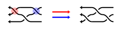 In a higher-categorical version of a prebraiding, these two witnesses for the braid relation need not be realized by the same 2-morphism. However, in the axiomatics of braided monoidal 2-categories, the cells witnessing these two proofs are equated by the so-called \(S_+=S_-\) relation of [BN96] (which was omitted in [KV94]). For a monoidal higher category, a prebraiding on the identity functor therefore does not imply the braid relations ([001P]), see also Remark 2.5.7, and in particular does not encode a braided monoidal (i.e. \(\mathbb E_2\)-)structure. In section 7, we will revisit this point and show that a prebraiding on the identity functor always encodes an \(\mathbb A_2 \otimes \mathbb E_1\)-structure, which differ in general from \(\mathbb E_2\)-structures.
We also want to introduce a relative notion of prebraiding, over a braided monoidal \(1\)-category:
Let \(\mathcal D\) be a braided monoidal \(1\)-category. Assume \(\mathcal C_1\) is a monoidal \(1\)-category, and \(\mathcal C_2\) is a monoidal category over \(\mathcal D\), i.e. equipped with a monoidal functor \(g\colon \mathcal C_2\rightarrow\mathcal D\). Let now \(F\colon \mathcal C_1 \rightarrow\mathcal C_2\) be a monoidal functor. Then we can consider \(C_1\) as a monoidal \(1\)-category over \(\mathcal D\), namely with respect to \(f \coloneqq g\circ F \colon \mathcal C_1 \rightarrow\mathcal D\), and \(F\) becomes a monoidal functor over \(\mathcal D\).
A prebraiding over \(\mathcal D\) on \(F \colon \mathcal C_1 \rightarrow\mathcal C_2\) is then defined to be a prebraiding on \(F\) as in Definition 2.4.1, satisfying the additional condition that \(g\) maps the prebraiding isomorphisms in \(\mathcal C_2\) to the given braiding isomorphisms in \(\mathcal D\).
More explicitly, with \(\mathcal D,\mathcal C_1,\mathcal C_2,F,g,f\) as in Definition 2.4.5, a prebraiding on \(F\) with components \(\beta_{x,y}\) is a prebraiding on \(F\) over \(\mathcal D\) if the isomorphism \[g \circ \beta_{x,y}\colon g(F(x)) \boxtimes g(F(y))\simeq g(F(x) \boxtimes F(y)) \rightarrow g(F(y) \boxtimes F(x)) \simeq g(F(y)) \boxtimes g(F(x))\] coincides with the given braiding isomorphism on \(\mathcal D\), i.e. with \(f(x) \boxtimes f(y) \rightarrow f(y)\boxtimes f(x)\) for all pairs of objects \(x,y\in\mathcal C_1\).
Let \(\mathcal A\) with \(g \colon \mathcal A\rightarrow \mathcal D\) be a monoidal \(1\)-category over \(\mathcal D\). Then a prebraiding over \(\mathcal D\) on the identity functor \(\mathrm{Id}\colon \mathcal A\rightarrow\mathcal A\) is a braided monoidal structure on \(\mathcal A\) with the property that \(g\) is braided monoidal in the sense of [Eti+15, Def. 8.1.7.].
For a monoidal functor \(F\colon \mathcal A\rightarrow\mathcal B\), we denote by \(\mathrm{PreBraid}(F)\) the set of prebraidings of \(F\) and for a monoidal category \(\mathcal A\), we denote by \(\mathrm{Braid}(\mathcal A)\coloneqq\mathrm{PreBraid}(\mathrm{Id}\colon \mathcal A\rightarrow\mathcal A)\) the set of compatible braidings on \(\mathcal A\). The relative versions of Definition 2.4.5 are denoted by \(\mathrm{PreBraid}_{/\mathcal D}(F\colon \mathcal A\rightarrow\mathcal B)\) and \(\mathrm{Braid}_{/\mathcal D}(\mathcal A)\) respectively.
2.5 Prebraiding for Soergel bimodules[001V]
We are now prepared to construct a prebraiding on the functor \(h_1 K_{\mathrm{loc}}\colon h_1 \mathrm{BSbim}\rightarrow h_1 \mathrm{K}^b_{\mathrm{loc}}(\mathrm{Sbim})\) from ([001D]).
For \(m,n\in \mathbb{N}\) let \(\beta_{m,n}\colon m+n\rightarrow n+m\) be the morphism in \(h_1 \mathrm{K}^b_{\mathrm{loc}}(\mathrm{Sbim})\) given by the chain homotopy class of the shifted Rouquier complex \((X_{m,n})\) defining the cabled crossing in Definition 2.2.7.
Theorem 2.5.2. (Prebraiding for Soergel bimodules).
The family of morphisms \(\beta_{m,n}\) from Definition 2.5.1 constitute a prebraiding on the functor \(h_1 K_{\mathrm{loc}}\colon h_1 \mathrm{BSbim}\rightarrow h_1 \mathrm{K}^b_{\mathrm{loc}}(\mathrm{Sbim})\).
Considering \(h_1 K_{\mathrm{loc}}\colon h_1 \mathrm{BSbim}\rightarrow h_1 \mathrm{K}^b_{\mathrm{loc}}(\mathrm{Sbim})\) as a functor over \(h_1\mathrm{DMor}^{\mathrm{poly}, \mathrm{gr-perf}}(\mathrm{mod}_k^{\mathbb{Z}})\) via the functor \(h_1H_{\mathrm{loc}}\colon h_1 \mathrm{K}^b_{\mathrm{loc}}(\mathrm{Sbim}) \rightarrow h_1\mathrm{DMor}^{\mathrm{poly}, \mathrm{gr-perf}}(\mathrm{mod}_k^{\mathbb{Z}})\), we obtain the following refined version:
Corollary 2.5.3. (Relative prebraiding on \(h_1 K_{\mathrm{loc}}\)).
The Rouquier complexes of cabled crossings define a prebraiding on \(h_1 K_{\mathrm{loc}}\colon h_1 \mathrm{BSbim}\rightarrow h_1 \mathrm{K}^b_{\mathrm{loc}}(\mathrm{Sbim})\) over \(h_1\mathrm{DMor}^{\mathrm{poly}, \mathrm{gr-perf}}(\mathrm{mod}_k^{\mathbb{Z}})\).
Proof.
By Remark 2.2.6, the braiding complexes are quasi-isomorphic to the associated permutation bimodules, concentrated in homological degree \(0\). As the permutation bimodules implement the symmetric braiding, this means that the braiding complexes constructed as (shifted) Rouquier complexes of the cabled crossings become the canonical symmetric braiding in \(h_1\mathrm{DMor}^{\mathrm{poly}, \mathrm{gr-perf}}(\mathrm{mod}_k^{\mathbb{Z}})\). ◻
The following result is the crucial naturality part for the proof of Theorem 2.5.2. The result is in fact stronger than needed, since it is a statement on the chain level.
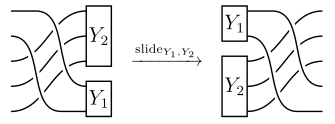
For any Bott–Samelson bimodule of the form \(Y=Y_1\boxtimes Y_2\) in \(\mathrm{BSbim}_m\boxtimes \mathrm{BSbim}_n\subset \mathrm{Sbim}_{m+n}\), there are homotopy equivalences of chain complexes in \(\mathrm{Ch}^b(\mathrm{Sbim}_{m+n})\): \[\begin{aligned} \mathrm{slide}_{Y_1,Y_2}\colon & X_{m,n} \circ_1Y \longrightarrow \mathrm{swap}_{m,n}(Y)\circ_1X_{m,n} \end{aligned}\]
We also use the notation \(\mathrm{slide}_{Y}\coloneqq\mathrm{slide}_{Y_1,Y_2}\), when \(m\) and \(n\) are clear from the context.
Proof of theorem 2.5.2.
theorem 2.5.4 indeed implies theorem 2.5.2. Namely it follows from Theorem 2.2.4 that the \(\beta_{m,n}\) are invertible and satisfy the hexagon axioms ([001L]) and thus form the components of a natural transformation \(\boxtimes\circ (h_1 K_{\mathrm{loc}}\times h_1 K_{\mathrm{loc}}) \Rightarrow \boxtimes^{\mathrm{op}}\circ (h_1 K_{\mathrm{loc}}\times h_1 K_{\mathrm{loc}})\) by Theorem 2.5.4. ◻
To establish theorem 2.5.4 we construct, after some preparation, the chain maps, which we then call slide maps, explicitly. For this we work with the Hecke category \(\mathcal{DS}_n\), i.e. the diagrammatical presentation of the monoidal \(1\)-category \(\mathrm{BSbim}_n\) from [EW16], [EK10]. The construction of the chain maps \(\mathrm{slide}_{Y_1,Y_2}\) proceeds in two steps. The first step is specific to the setting of Bott–Samelson and Soergel bimodules and uses \(\mathcal{DS}\). It establishes the existence of atomic slide chain maps, namely \(\mathrm{slide}_{\mathbf{1}_1,B_1}\) for \((m,n)=(1,2)\) and \(\mathrm{slide}_{B_1,\mathbf{1}_1}\) for \((m,n)=(2,1)\); see Lemma 2.5.5. The second step uses that every Bott–Samelson bimodule is a composition (monoidal and horizontal) of Bott–Samelson bimodules on two strands, and so knowing the atomic slide chain maps is sufficient to construct general slide maps along the following scheme: 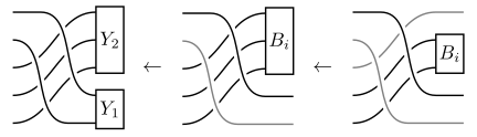 Essentially the same argument would work for any monoidal bicategory generated by a single object and one endomorphism of its tensor square.
To formulate the statements, we need at least a rough description of the Hecke category \(\mathcal{DS}_n\) and the fact that it is equivalent to \(\overline{\mathrm{BSbim}}^{\mathrm{gr}}_n\) as graded monoidal \(k\)-linear category. For details we refer to [EW16], [EK10]. Each simple reflection \(s_i\in S_n\) is encoded by a colour. Objects in \(\mathcal{DS}_n\) are finite ordered sequences of such colours and they encode the Bott–Samelson bimodules in the form ([000N]) (with \(j=0\) since we consider \(\overline{\mathrm{BSbim}}^{\mathrm{gr}}_n\)). For instance if \(n=2\) and we encode \(s_1\) as red and \(s_2\) as blue, then the Bott–Samelson bimodule \(B_{\mathbf{i}}\) from ([000N]) is encoded as a sequence of colors red and blue according to \({\mathbf{i}}\), for instance \({\mathbf{i}}=(1,1,2,1,1)\) corresponds to the object given by the color sequence \((red, red, blue, red, red)\). Morphisms in \(\mathcal{DS}_n\) are \(k\)-linear combinations of isotopy classes of certain decorated graphs embedded in the plane. A morphism from \(B_{\mathbf{i}}\) to \(B_{\mathbf{i}'}\) will have the colour sequence for \({\mathbf{i}}\) as bottom boundary and that for \({\mathbf{i}}'\) at the top boundary; for instance the first two diagrams in ([0023]) represent morphism from \((2,2)\) to \((2)\) and vice versa, the third goes from the unit to \((2)\), etc.
The monoidal structure is given on objects by concatenating sequences and, on morphisms, by (the bilinear extension of) placing diagrams horizontally next to each other. The composition of morphisms is, likewise, given by (the bilinear extension of) stacking diagrams on top of each other. The empty sequence is the unit object.
Apart from multiplication with polynomials, the generating morphisms (in the monoidal sense) are exactly the following, where blue represents any color/number which is neighbored to red and not neighbored to orange. 
For the rest of this section we identify \(\mathrm{BSbim}_n\) with \(\mathcal{DS}_n\) as monoidal \(1\)-categories (via \(\overline{\mathrm{BSbim}}^{\mathrm{gr}}_n\)) and perform computations using the diagrammatic calculus.
The Rouquier complexes ([000Z]) are translated into the diagrammatics as  where we encode \(s_i\) by blue. (Instead of remembering the grading shifts from ([000Z]), it is more convenient in the diagrammatic setting to consider the maps as homogeneous of degree one). To keep track of the monoidal unit (corresponding to \(R\)) appearing in the complexes, we mostly indicate them by a colored dot as shown in ([0024]).
There are slide chain maps 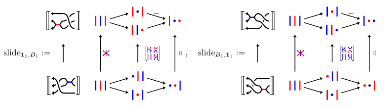 which are invertible up to homotopy. The inverses are given by the chain maps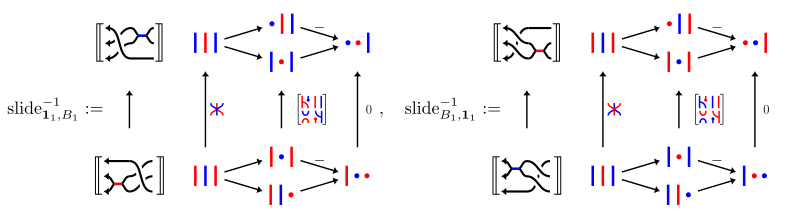
Proof.
The proof is given by an explicit calculation. As an example (the remaining cases are checked analogously) we show that \(\mathrm{slide}^{-1}_{\mathbf{1}_1,B_1}\circ\; \mathrm{slide}_{\mathbf{1}_1,B_1}\) is homotopic to the identity by computing their difference and exhibiting an explicit null-homotopy: 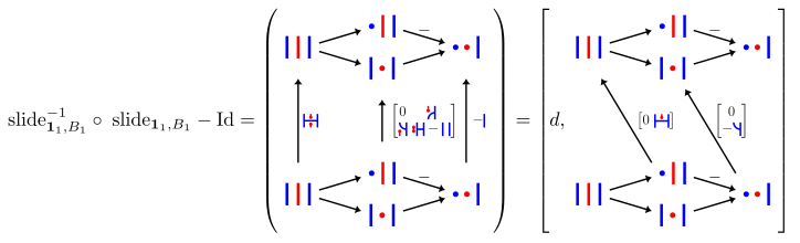 ◻
◻
Observe that the relevant chain complexes and chain maps are for the two cases are related by swapping the colours red and blue.
Readers familiar with the chain maps between Rouquier complexes associated to a Reidemeister III move will recognize the atomic slide chain maps as filtrations-preserving pieces of the former, see e.g. [MWW22, (3.3) and (3.4)].
Now that we have obtained the atomic slide chain maps in lemma 2.5.5, we can construct all remaining slide chain maps in an essentially formal way.
Proof of Theorem 2.5.4.
We will focus on the version for the positive cabled crossing, since the other one is analogous. First, we reduce to the case when the object \(Y=Y_1\boxtimes Y_2\) is a generating object of \(\mathrm{BSbim}_m\boxtimes \mathrm{BSbim}_n\). Otherwise, we can decompose into generators: \[Y_1\boxtimes Y_2= (Y_1\boxtimes \mathbf{1}) \circ_1(\mathbf{1}\boxtimes Y_2) = (B_{i_1}\boxtimes \mathbf{1}) \circ_1\cdots \circ_1(B_{i_a}\boxtimes \mathbf{1}) \circ_1(\mathbf{1} \boxtimes B_{j_1})\circ_1\cdots \circ_1(\mathbf{1} \boxtimes B_{j_b})\] and define \[\begin{aligned} \mathrm{slide}_{Y_1,\mathbf{1}}&:= (\mathrm{id}_{\mathrm{swap}_{m,n}(B_{i_1}\circ_1\cdots \circ_1B_{i_{a-1}} \boxtimes \mathbf{1})}\circ_1\mathrm{slide}_{B_{i_{a}},\mathbf{1}}) \circ_2\cdots \circ_2 (\mathrm{slide}_{B_{i_{1}},\mathbf{1}} \circ_1\mathrm{id}_{B_{i_1}\circ_1\cdots \circ_1B_{i_{a-1}} \boxtimes \mathbf{1}}) \\ \mathrm{slide}_{\mathbf{1},Y_2}&:= (\mathrm{id}_{\mathrm{swap}_{m,n}(\mathbf{1}\boxtimes B_{j_1}\circ_1\cdots \circ_1B_{j_{b-1}})}\circ_1\mathrm{slide}_{\mathbf{1}, B_{j_{b}}}) \circ_2\cdots \circ_2 (\mathrm{slide}_{\mathbf{1}, B_{j_{1}}} \circ_1\mathrm{id}_{\mathbf{1}\boxtimes B_{j_1}\circ_1\cdots \circ_1B_{j_{b-1}}}) \\ \mathrm{slide}_{Y_1,Y_2} &:= (\mathrm{id}_{\mathrm{swap}_{m,n}(Y_1\boxtimes \mathbf{1})} \circ_1\mathrm{slide}_{\mathbf{1},Y_2}) \circ_2(\mathrm{slide}_{Y_1,\mathbf{1}} \circ_1\mathrm{id}_{Y_2}) \end{aligned}\]
Now we turn to defining \(\mathrm{slide}_{B,\mathbf{1}_n}\) and \(\mathrm{slide}_{\mathbf{1}_m,B}\), where \(B\) is one of the generating Bott–Samelson bimodules. Here we place subscripts to distinguish the identity bimodules. We first consider the latter situation and reduce it to the case \(m=1\), where the cabled crossing is a Coxeter braid. Indeed, suppose that \(m>1\), then we use the first equality from Lemma 2.2.8 to define \(\mathrm{slide}_{\mathbf{1}_m,B}\) to be the composite: \[\begin{gathered} \nonumber \big((\mathrm{slide}_{\mathbf{1}_1,B}\boxtimes \mathrm{id}_{\mathbf{1}_{m-1}}) \circ_1\cdots \circ_1 \mathrm{id}_{\mathbf{1}_{m-1-i} \boxtimes X_{1,n}\boxtimes\mathbf{1}_{i}} \circ_1\cdots \circ_1 \mathrm{id}_{\mathbf{1}_{m-1}\boxtimes X_{1,n}}\big) \circ_2\cdots \\ \circ_2\big(\mathrm{id}_{X_{1,n}\boxtimes \mathbf{1}_{m-1}} \circ_1\cdots \circ_1 (\mathrm{id}_{\mathbf{1}_{m-1-i}} \boxtimes \mathrm{slide}_{\mathbf{1}_1,B}\boxtimes\mathrm{id}_{\mathbf{1}_{i}}) \circ_1\cdots \circ_1 \mathrm{id}_{\mathbf{1}_{m-1}\boxtimes X_{1,n}}\big) \circ_2\cdots\\ \nonumber \circ_2\big(\mathrm{id}_{X_{1,n}\boxtimes \mathbf{1}_{m-1}} \circ_1\cdots \circ_1 \mathrm{id}_{\mathbf{1}_{m-1-i} \boxtimes X_{1,n}\boxtimes\mathbf{1}_{i}} \circ_1\cdots \circ_1 (\mathrm{id}_{\mathbf{1}_{m-1}}\boxtimes \mathrm{slide}_{\mathbf{1}_1,B}) \big) \end{gathered}\] For the other case, we first choose chain maps \(\varphi\) and \(\varphi^{-1}\) realising the first homotopy equivalence in Lemma 2.2.8. Then we define \(\mathrm{slide}_{B,\mathbf{1}_n}\) as the composition: \[\begin{gathered} \nonumber \varphi^{-1} \circ_2\big((\mathbf{1}_{n-1}\boxtimes \mathrm{slide}_{B,\mathbf{1}_1}) \circ_1\cdots \circ_1 \mathrm{id}_{\mathbf{1}_{i} \boxtimes X_{m,1}\boxtimes\mathbf{1}_{n-1-i}} \circ_1\cdots \circ_1 \mathrm{id}_{X_{m,1}\boxtimes \mathbf{1}_{n-1}}\big) \circ_2\cdots \\ \circ_2\big(\mathrm{id}_{\mathbf{1}_{n-1}\boxtimes X_{m,1}} \circ_1\cdots \circ_1 (\mathrm{id}_{\mathbf{1}_{i}} \boxtimes \mathrm{slide}_{B,\mathbf{1}_1}\boxtimes\mathrm{id}_{\mathbf{1}_{n-1-i}}) \circ_1\cdots \circ_1 \mathrm{id}_{X_{m,1}\boxtimes \mathbf{1}_{n-1}}\big) \circ_2\cdots \\ \nonumber \circ_2\big(\mathrm{id}_{\mathbf{1}_{n-1}\boxtimes X_{m,1}} \circ_1\cdots \circ_1 \mathrm{id}_{\mathbf{1}_{i} \boxtimes X_{m,1}\boxtimes\mathbf{1}_{n-1-i}} \circ_1\cdots \circ_1 (\mathrm{slide}_{B,\mathbf{1}_1}\boxtimes \mathbf{1}_{n-1}) \big)\circ_2\varphi \end{gathered}\] It remains to construct \(\mathrm{slide}_{\mathbf{1}_1,B_i}\) and \(\mathrm{slide}_{B_j,\mathbf{1}_1}\) where \(B_i\) is a generating object of \(\mathrm{BSbim}_n\) and \(B_j\) is a generating object of \(\mathrm{BSbim}_m\). Now we reduce this problem to the cases when \(n=2\) and \(m=2\) respectively. We define \(\mathrm{slide}_{\mathbf{1}_1,B_i}\) as the composite: \[\begin{aligned} F(\sigma_{n}\cdots\sigma_{1}) \circ_1B_i =& F(\sigma_{n}\cdots\sigma_{i+1})\circ_1F(\sigma_{i}\sigma_{i-1})\circ_1F(\sigma_{i-2}\cdots\sigma_{1})\circ_1B_i \\ \rightarrow &F(\sigma_{n}\cdots\sigma_{i+1})\circ_1F(\sigma_{i}\sigma_{i-1}) \circ_1B_i \circ_1F(\sigma_{i-2}\cdots\sigma_{1}) \\ \xrightarrow{\mathrm{slide}} &F(\sigma_{n}\cdots\sigma_{i+1})\circ_1B_{i-1} \circ_1F(\sigma_{i}\sigma_{i-1}) \circ_1F(\sigma_{i-2}\cdots\sigma_{1}) \\ \rightarrow& B_{i-1} \circ_1F(\sigma_{n}\cdots\sigma_{i+1})\circ_1F(\sigma_{i}\sigma_{i-1}) \circ_1F(\sigma_{i-2}\cdots\sigma_{1})\\ =& B_{i-1} \circ_1F(\sigma_{n}\cdots\sigma_{1}) \end{aligned}\] where the unlabelled maps are far-commutativity isomorphisms and the labelled arrow is given by \(\mathrm{id}\circ_1\mathrm{slide}_{\mathbf{1}_1,B_1} \circ_1\mathrm{id}\), which is determined by the \(n=2\) case. The reduction of \(\mathrm{slide}_{B_j,\mathbf{1}_1}\) to the case \(m=2\) is completely analogous.
Thus we reduced the problem to the statement from Lemma 2.5.5. By construction, all slide maps constructed in this proof are homotopy equivalences. ◻
In Remarks 2.4.3 and 2.4.4 we have observed that a prebraiding need not satisfy the braid relation, and that the braid relation in prebraidings on identity functors can be verified in two ways using naturality. On the level of the homotopy category of Soergel bimodules, this is reflected in the fact, that the chain maps implementing the homotopy equivalence corresponding to a braid relation live in a 2-dimensional space [EK10, Section 3, Reidemeister 3 generators]. One dimension is encoding an overall non-zero scaling. Even after fixing this, there exists however a 1-dimensional affine subspace of representatives of the same homotopy class of chain maps. Two distinct (and thus spanning) points in this subspace can be built from slide chain maps, analogously to the two ways of establishing the braid relation in Remark 2.4.4.
We used Rouquier canonicity to ensure here the independence (up to canonical isomorphism) of our choices in the construction of the prebraiding on \(h_1 K_{\mathrm{loc}}\) in Theorem 2.5.2. For the rest of the paper it would be enough to make one of the choices and establish the prepraiding using only the monoidality of \(h_1 K_{\mathrm{loc}}\). The desired independence of choices (and in fact also Rouqiuer canonicity itself) could then be deduced from the existence statement in corollary 8.2.2.
2.6 Centralizers and prebraidings[002C]
In the following, given a monoidal \(1\)-category \(\mathcal C\), we will identify \(1\boxtimes x\) and \(x\boxtimes 1\) with \(x\) for any object \(x\in\mathcal C\), see [Eti+15, Rk. 2.2.9], and will suppress writing associators, as they can be recovered from context.
Let \(\mathcal A\) and \(\mathcal B\) be monoidal \(1\)-categories and let \(F\colon\mathcal A\rightarrow\mathcal B\) be a monoidal functor. The centralizer \(Z(F)\) of \(F\) is the following category:
Its objects are pairs \((b,\gamma)\) of an object \(b\in\mathcal B\) and a natural isomorphism \[\gamma=\gamma_-\colon b\boxtimes F(-)\rightarrow F(-)\boxtimes b\] of functors from \(\mathcal A\) to \(\mathcal B\), called half-braiding, which satisfies the following two compatibility conditions with respect to the monoidal structure of \(\mathcal A\). Firstly, for any \(a_1,a_2\in\mathcal A\), the isomorphism \(\gamma_{a_1 \boxtimes a_2} \colon b \boxtimes F(a_1 \boxtimes a_2) \rightarrow F(a_1 \boxtimes a_2) \boxtimes b\) equals the composite \[b\boxtimes F(a_1\boxtimes a_2)\xrightarrow{\simeq} b\boxtimes F(a_1)\boxtimes F(a_2)\xrightarrow{(\mathrm{id}\boxtimes \gamma_{a_2})\circ (\gamma_{a_1}\boxtimes\mathrm{id})} F(a_1)\boxtimes F(a_2)\boxtimes b\xrightarrow{\simeq} F(a_1\boxtimes a_2) \boxtimes b,\] and secondly \[\gamma_{1_{\mathcal A}} = \left(b\boxtimes F(1_{\mathcal A})\xrightarrow{\simeq} b\boxtimes 1_{\mathcal B}=1_{\mathcal B}\boxtimes b\xrightarrow{\simeq}F(1_{\mathcal A})\boxtimes b\right).\]
Its morphisms are morphisms in \(\mathcal B\) that are compatible with the half-braidings as follows: \[\mathrm{Hom}_{Z(F)}((b,\gamma),(b',\gamma'))=\{f\in\mathrm{Hom}_{\mathcal B}(b,b')\mid \gamma'_a\circ (f\boxtimes\mathrm{id})=(\mathrm{id}\boxtimes f)\circ\gamma_a \colon b\boxtimes F(a)\rightarrow F(a)\boxtimes b\}.\]
The composition is inherited from \(\mathcal B\).
The category \(Z(F)\) is monoidal with \((b,\gamma)\boxtimes (b,\gamma')\coloneqq (b\boxtimes b',\gamma\boxtimes\mathrm{id}\circ\mathrm{id}\boxtimes\gamma')\) on objects, and with the tensor product from \(\mathcal B\) on morphisms. The unit object \(1_{Z(F)}\in Z(F)\) is \((1_{\mathcal B}\in\mathcal B, \gamma)\) with \(\gamma_a\colon 1\boxtimes F(a)=F(a)=F(a)\boxtimes 1\). We leave the coherence isomorphisms and their compatibility to the reader.
In case \(\mathcal A=\mathcal B\) and \(F= \mathrm{id}_{\mathcal A}\) is the identity functor, the centralizer \(Z(\mathrm{id}_{\mathcal A})\) is the Drinfeld center \(Z(A)\) of \(\mathcal A\), [Eti+15, Def. 7.13.1]. The generalized hexagon axiom above turns then into the familiar hexagon diagram [Eti+15, (7.41)]. Centralizers, as generalizations of Drinfeld centers, appear already in [Maj91, §3].
For a monoidal functor \(F\colon \mathcal A\rightarrow\mathcal B\), we define the monoidal evaluation functor \[\mathrm{ev}\colon Z(F) \times \mathcal A\rightarrow\mathcal B\] to send an object \(((b,\gamma),a)\) to \(b\boxtimes F(a)\), and a morphism \((f,g)\) to \(f\boxtimes F(g)\). The monoidal structure isomorphisms \[\mathrm{ev}\left(((b,\gamma),a)\boxtimes((b',\gamma'),a')\right)\simeq \mathrm{ev}\left((b,\gamma),a\right)\boxtimes \mathrm{ev}\left((b',\gamma'),a')\right) \quad(\text{for } a,a'\in\mathcal A,(b,\gamma),(b',\gamma')\in Z(F))\] are given by \(b\boxtimes b'\boxtimes F(a\boxtimes a')\simeq b\boxtimes b'\boxtimes F(a)\boxtimes F(a') \xrightarrow{\mathrm{id}\boxtimes\gamma'_a\boxtimes\mathrm{id}} b\boxtimes F(a)\boxtimes b'\boxtimes F(a')\). The defining properties of \(\gamma'\) and the monoidality of \(F\) ensure that the necessary compatibilities hold, so that we indeed get a monoidal functor.
Together with the unit \(1_{Z(F)} \in Z(F)\) and \(F \colon \mathcal A\rightarrow\mathcal B\), the evaluation functor fits into the following commuting diagram of monoidal functors: 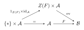
In example 7.4.4, we will discuss the universal property satisfied by \(Z(F)\) with its monoidal evaluation functor.
The functor \(\mathrm{ev}\) is completely determined by the monoidal functor \[\mathrm{ev}_{1_{\mathcal A}} \coloneqq \mathrm{ev}(-, 1_{\mathcal A}) \colon Z(F) \rightarrow\mathcal B,\] which sends an object \((b, \gamma)\in Z(F)\) to the underlying object \(b\) and a morphism in \(Z(F)\) to the underlying morphism in \(\mathcal B\). In these terms, \(\mathrm{ev}(-, ?) = \mathrm{ev}_{1_{\mathcal A}}(-) \boxtimes F(?)\).
We obtain a classification of prebraidings on a monoidal functor \(F\), Definitions 2.4.1 and 2.4.8, in terms of the centralizer \(Z(F)\) of \(F\):
Let \(F\colon \mathcal A\rightarrow\mathcal B\) be a monoidal functor between monoidal \(1\)-categories. Then the following are equivalent:
the set \(\mathrm{PreBraid}(F)\) of prebraidings on \(F\);
the set of strict monoidal factorizations of \(F\) through \(\mathrm{ev}_{1_{\mathcal A}} \colon Z(F) \rightarrow\mathcal B\), i.e. the set of monoidal functors \(s\colon \mathcal A\rightarrow Z(F)\) such that \(\mathrm{ev}_{1_{\mathcal A}} \circ s=F\).
the 1-groupoid of weak monoidal factorizations of \(F\) through \(\mathrm{ev}_{1_{\mathcal A}} \colon Z(F) \rightarrow\mathcal B\), i.e. the groupoid whose objects are pairs \((s,\eta)\) of a monoidal functor \(s \colon \mathcal A\rightarrow Z(F)\) and a monoidal natural isomorphism \(\eta \colon \mathrm{ev}_{1_{\mathcal A}} \circ s \Rightarrow F\) and whose morphisms \((s, \eta) \rightarrow(s', \eta')\) are monoidal natural isomorphisms \(\mu \colon s\Rightarrow s'\) such that \[\left( \mathrm{ev}_{1_{\mathcal A}} \circ s \xRightarrow{\mathrm{ev}_{1_{\mathcal A}} \circ \mu} \mathrm{ev}_{1_{\mathcal A}} \circ s' \xRightarrow{\eta'} F \right)=\left( \mathrm{ev}_{1_{\mathcal A}} \circ s \xRightarrow{\eta}F\right).\]
Proof.
For the equivalence between ([002H]) and ([002I]), note that a factorization \(s\) must send, on the level of objects, \(x\) to \((F(x),\gamma)\) for some \(\gamma\), and on the level of morphisms \(f\) to \(F(f)\). The isomorphisms used for a prebraiding \(\beta\) uniquely define the isomorphisms encoded in a possible \(\gamma\). The second hexagon axiom from prebraidings ([001L]) translates into the required properties of \(\gamma\), whereas the first hexagon translates into the monoidality of \(s\).
The equivalence between ([002I]) and ([002J]) follows from abstract-nonsense: Recall that a monoidal functor \(F:\mathcal X\rightarrow\mathcal Z\) between monoidal \(1\)-categories is called an isofibration if for all isomorphisms \(\gamma \colon z \rightarrow z'\) in \(\mathcal Z\) and \(x \in \mathcal X\) with \(F(x) = z\), there exists an isomorphism \(\mu \colon x\rightarrow x'\) with \(F(\mu) = \gamma\). It is then an exercise to show that if \(F \colon \mathcal X\rightarrow\mathcal Z\) is a monoidal functor which is a faithful isofibration and \(G\colon \mathcal Y\rightarrow\mathcal Z\) is another monoidal functor, the groupoid of weak monoidal factorizations, i.e. of pairs \((s, \eta)\) of a monoidal functor \(s \colon \mathcal Y\rightarrow\mathcal X\) and a monoidal natural isomorphism \(F \circ s \simeq G\) is equivalent to a discrete groupoid isomorphic to the set of strict monoidal factorizations, i.e. the set of monoidal functors \(s\) such that \(F \circ s = G\). The equivalence between ([002I]) and ([002J]) then follows since \(\mathrm{ev}_{1_{\mathcal A}} \colon Z(f) \rightarrow\mathcal B\) is indeed a faithful isofibration. ◻
The special case \(F=\mathrm{id}_\mathcal A\) for a monoidal category \(\mathcal A\) gives a bijection \[\begin{aligned} \mathrm{Braid}(\mathcal A) &\simeq& \{\text{Monoidal sections }\mathcal A\rightarrow Z(\mathcal A) \text{ of }\mathrm{ev}_{1_{\mathcal A}}\colon Z(\mathcal A)\rightarrow\mathcal A\}. \end{aligned}\]
Original source: arXiv:2401.02956v2
Original source · 2401.02956v2